Excel Template for a Loan Amortization Schedule

1.

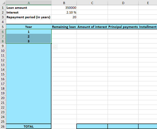
The first thing you do is to enter the relevant numbers for your loan:

2.

The next thing you do is to make the “skeleton” of the table above the repayment of the amortizing loan. This table need the columns “year”, “remaining loan”, “amount of interest”, “principal payments” and “installment”.

You need to make a row for the years 1 through 20. Instead of making a row for all the integers manually, you can use a clever feature in Excel that does the job for you. Enter the numbers 1, 2, 3 as shown below, and then mark the cells.

Then press and hold the little green square in the bottom right corner of cell A8 and pull it all the way down till you see the number 20. (A small gray square will count the number of rows you pull it).

3.

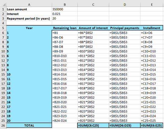
The remaining loan the first year is the original loan amount. You can enter $$350000$ in cell B6, but you have already typed the number in cell B1 in the spreadsheet. A more elegant solution is to use the functionality of the spreadsheet by typing in cell B6:

=B1

This way you only need to change the value of cell B1 if you want to change the original loan amount.

The interest amount of year 1 will be the same as the remaining loan of year 1 multiplied by the interest. To calculate the interest of year 1, enter into cell C6:

=B6*$B$2

Note! The $-sign before the letter- and number-coordinates of the cell B2, is to use the functionality of the spreadsheet that allows you to copy formulas. This will be explained more closely below.

The principal payments of an amortizing loan are always equal. You can easily calculate the amount

$$\begin{array}{llll}\hfill \text{Principal payment}& =\frac{\text{Loan amount}}{\text{Number of installments}}& \hfill & \\ \hfill & =\frac{350000\text{kr}}{20}& \hfill & \\ \hfill & =17500\text{kr}& \hfill & \end{array}$$

You can write $$17500$ in the cell for principal payment year 1, but if you wish to change the original loan amount, you need to change the installment cell as well. Therefore, it can be wise to write the calculation of the installment in the cell of the installment D6. So, in cell D6 you write:

=$B$1/$B$3

The installment amount is the interest amount + principal payment. In cell E6, where the installment amount of year 1 is, write:

=C6+D6

You’ve now spent some time on just filling out a few cells, but soon, you’ll experience the spreadsheets magic! The last part is to enter the remaining loan of year 2 is going. The calculation goes as follows:

$$\text{Remaining loan after 2 years}=\text{Remaining loan after 1 year}-\text{Installment year 1}$$

In cell  B7, write:

=B6-E6

4.

This is when the fun starts! You are now to copy the formula for remaining loan by marking B7. Then you pull the small green square and pull it all the way down to the 20th year. The way Excel thinks is that the formula in the marked cell is to be copied and performed in the cells below that belong to the same column. Excel sees that the formula in the marked cell consists of subtracting the number in the cell that’s one cell up and two to the right, from the number in the cell above.

Note! Every row depends on the row above, so you may notice that the numbers in your spreadsheet could be incorrect until you are done with all the columns.

Now you can copy the formula inD6 in all the cells below in the installment column. The difference between the installment column and the remaining loan column is that you always want to refer to the columns B1 and B3 in the installment column. To let Excel know that you always want to use these two cells instead of moving downwards, write the $-sign before the letter- and number coordinates of the cells. So again, mark cell D6 and pull it down to the 20th year.

Now you can see that the numbers in the remaining loan column are correct.

Do the same with the columns for amount of interest and principal payment. That is, mark C6 and pull it down to year 20, and then mark E6 and do the same. Notice that in the column for amount of interest you want to use the remaining loan column in the same row, but always the same interest (B2). Therefore, use the $-sign when referring to the interest in the formula in C6, but not when referring to the remaining loan.

5.

Finally, it can be good to sum the amount of interest, installments and principal payment respectively cell C26, D26 and E26. In  C26, write:

=SUM(C6:C25)

Do the equivalent for the columns for installment and principal payment. The final spreadsheet will then look like this:

And with the formulas:

The sum of the installments should be equal to the loan amount, and you can see that this is the case here. The sum of the interest amount will equal to what you have paid in interest, which is $$77175$, and the sum of the principal payments are all the money you have returned to the bank, which is $$427175$. In other words, an amortizing loan of $$350000$ cost you $$427175$ after 20 years.